Code Cells (nbsphinx)#

This page demonstrates a notebook converted with nbsphinx, so you can see how it looks with the PyData Sphinx theme. Note: it should look basically the same converted with MyST-NB.

This document is a modified copy of an example notebook in the nbsphinx docs. The original source is in the nbsphinx GitHub repo.

Code, Output, Streams#

An empty code cell:

[ ]:

Two empty lines:

[ ]:

Leading/trailing empty lines:

[1]:

# 2 empty lines before, 1 after

A simple output:

[2]:

6 * 7

[2]:

The standard output stream:

[3]:

print("Hello, world!")

Hello, world!

Normal output + standard output

[4]:

print("Hello, world!")
6 * 7

Hello, world!

[4]:

Normal output comes last. When both standard error and output are present, which one comes first can vary by kernel.

[5]:

import sys


print("I'll appear on the standard error stream", file=sys.stderr)
print("I'll appear on the standard output stream")
"I'm the 'normal' output"

I'll appear on the standard output stream

I'll appear on the standard error stream

[5]:

"I'm the 'normal' output"

Note

Using the IPython kernel, the order is actually mixed up, see ipython/ipykernel#280.

Long input and output

[6]:

"Lorem ipsum dolor sit amet, consectetur adipiscing elit, sed do eiusmod tempor incididunt ut labore et dolore magna aliqua. Ut enim ad minim veniam, quis nostrud exercitation ullamco laboris nisi ut aliquip ex ea commodo consequat. Duis aute irure dolor in reprehenderit in voluptate velit esse cillum dolore eu fugiat nulla pariatur. Excepteur sint occaecat cupidatat non proident, sunt in culpa qui officia deserunt mollit anim id est laborum."  # NOQA: E501

[6]:

'Lorem ipsum dolor sit amet, consectetur adipiscing elit, sed do eiusmod tempor incididunt ut labore et dolore magna aliqua. Ut enim ad minim veniam, quis nostrud exercitation ullamco laboris nisi ut aliquip ex ea commodo consequat. Duis aute irure dolor in reprehenderit in voluptate velit esse cillum dolore eu fugiat nulla pariatur. Excepteur sint occaecat cupidatat non proident, sunt in culpa qui officia deserunt mollit anim id est laborum.'

Error / traceback

[7]:

traceback  # NOQA: F821

---------------------------------------------------------------------------
NameError                                 Traceback (most recent call last)
Cell In[7], line 1
----> 1 traceback  # NOQA: F821

NameError: name 'traceback' is not defined

Special Display Formats#

Local Image Files#

[8]:

from IPython.display import Image


i = Image(filename="images/notebook_icon.png")
i

[8]:

[9]:

display(i)

Image URLs#

PNG format

[11]:

Image(url="https://www.python.org/static/img/python-logo-large.png")

[11]:

PNG format, embed=True

[12]:

Image(url="https://www.python.org/static/img/python-logo-large.png", embed=True)

[12]:

SVG format

[13]:

Image(url="https://jupyter.org/assets/homepage/main-logo.svg")

[13]:

Math#

[14]:

from IPython.display import Math


eq = Math(r"\int\limits_{-\infty}^\infty f(x) \delta(x - x_0) dx = f(x_0)")
eq

[14]:

$\displaystyle \int\limits_{-\infty}^\infty f(x) \delta(x - x_0) dx = f(x_0)$

[15]:

display(eq)

$\displaystyle \int\limits_{-\infty}^\infty f(x) \delta(x - x_0) dx = f(x_0)$

[16]:

from IPython.display import Latex


Latex(
    r"A lot of extra text "
    r"to test wrapping "
    r"when rendered to HTML. "
    r"This is an equation: $a^2 + b^2 = c^2$"
)

[16]:

A lot of extra text to test wrapping when rendered to HTML. This is an equation: $a^2 + b^2 = c^2$

Some elements are repeated in the following equation to make it longer. This makes it easier to test whether the equation looks good on a mobile screen, for example, where the width of the equation does not fit within the width of the screen:

[17]:

%%latex
\begin{equation}
\int\limits_{-\infty}^\infty f(x) \delta(x - x_0) \delta(x - x_0) \delta(x - x_0) \delta(x - x_0) \delta(x - x_0) \delta(x - x_0) dx = f(x_0)
\end{equation}

\begin{equation} \int\limits_{-\infty}^\infty f(x) \delta(x - x_0) \delta(x - x_0) \delta(x - x_0) \delta(x - x_0) \delta(x - x_0) \delta(x - x_0) dx = f(x_0) \end{equation}

Plots#

Note

Make sure to use at least version 0.1.6 of the matplotlib-inline package (which is an automatic dependency of the ipython package).

By default, the plots created with the “inline” backend have the wrong size. More specifically, PNG plots (the default) will be slightly larger than SVG and PDF plots.

This can be fixed easily by creating a file named matplotlibrc (in the directory where your Jupyter notebooks live, e.g. in this directory: matplotlibrc and adding the following line:

figure.dpi: 96

If you are using Git to manage your files, don’t forget to commit this local configuration file to your repository. Different directories can have different local configurations. If a given configuration should apply to multiple directories, symbolic links can be created in each directory.

For more details, see Default Values for Matplotlib’s “inline” Backend.

By default, plots are generated in the PNG format. In most cases, it looks better if SVG plots are used for HTML output and PDF plots are used for LaTeX/PDF. This can be achieved by setting nbsphinx_execute_arguments in your conf.py file like this:

nbsphinx_execute_arguments = [
    "--InlineBackend.figure_formats={'svg', 'pdf'}",
]

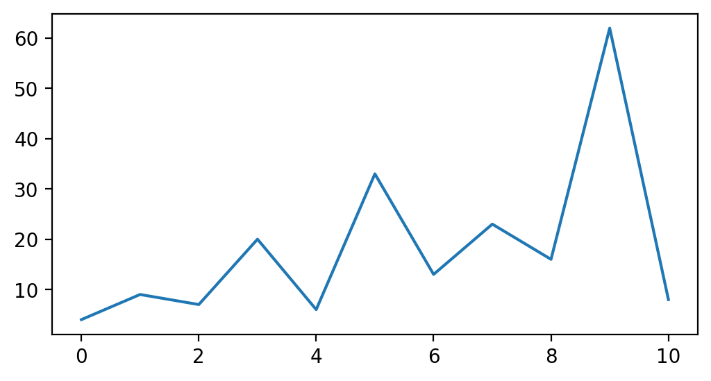
In the following example, nbsphinx should use an SVG image in the HTML output and a PDF image for LaTeX/PDF output (other Jupyter clients like JupyterLab will still show the default PNG format).

[18]:

import matplotlib.pyplot as plt

[19]:

%config InlineBackend.figure_formats = ['svg']

[20]:

fig, ax = plt.subplots(figsize=[6, 3])
ax.plot([4, 9, 7, 20, 6, 33, 13, 23, 16, 62, 8]);

For comparison, this is how it would look in PNG format …

[21]:

%config InlineBackend.figure_formats = ['png']

[22]:

fig

[22]:

… and in 'png2x' (a.k.a. 'retina') format:

[23]:

%config InlineBackend.figure_formats = ['png2x']

[24]:

fig

[24]:

Pandas Dataframes#

Pandas dataframes should be displayed as nicely formatted HTML tables (if you are using HTML output).

[25]:

import numpy as np
import pandas as pd

[26]:

df = pd.DataFrame(
    np.random.randint(0, 100, size=[10, 4]),
    columns=[r"$\alpha$", r"$\beta$", r"$\gamma$", r"$\delta$"],
)
df

[26]:

	$\alpha$	$\beta$	$\gamma$	$\delta$
0	39	3	53	0
1	30	83	32	99
2	47	28	1	29
3	97	67	13	61
4	15	90	1	7
5	51	67	27	68
6	72	22	47	18
7	12	76	14	70
8	57	20	98	87
9	3	97	25	31

Markdown Content#

[29]:

from IPython.display import Markdown

[30]:

md = Markdown("""
# Markdown

It *should* show up as **formatted** text
with things like [links] and images.

[links]: https://jupyter.org/

![Jupyter notebook icon](images/notebook_icon.png)

## Markdown Extensions

There might also be mathematical equations like
$a^2 + b^2 = c^2$
and even tables:

A     | B     | A and B
------|-------|--------
False | False | False
True  | False | False
False | True  | False
True  | True  | True

""")
md

[30]:

Markdown#

It should show up as formatted text with things like links and images.

Jupyter notebook icon

Markdown Extensions#

There might also be mathematical equations like $a^2 + b^2 = c^2$ and even tables:

A	B	A and B
False	False	False
True	False	False
False	True	False
True	True	True

YouTube Videos#

[31]:

from IPython.display import YouTubeVideo

YouTubeVideo("9_OIs49m56E")

[31]:

Interactive Widgets (HTML only)#

The basic widget infrastructure is provided by the ipywidgets module. More advanced widgets are available in separate packages, see for example https://jupyter.org/widgets.

The JavaScript code which is needed to display Jupyter widgets is loaded automatically (using RequireJS). If you want to use non-default URLs or local files, you can use the nbsphinx_widgets_path and nbsphinx_requirejs_path settings.

[32]:

import ipywidgets as w

[33]:

slider = w.IntSlider()
slider.value = 42
slider

[33]:

A widget typically consists of a so-called “model” and a “view” into that model.

If you display a widget multiple times, all instances act as a “view” into the same “model”. That means that their state is synchronized. You can move either one of these sliders to try this out:

[34]:

slider

[34]:

You can also link different widgets.

Widgets can be linked via the kernel (which of course only works while a kernel is running) or directly in the client (which even works in the rendered HTML pages).

Widgets can be linked uni- or bi-directionally.

Examples for all 4 combinations, all linked to the slider in the previous code cell, are shown here:

[35]:

# requires kernel, bi-directional
link = w.IntSlider(description="link")
w.link((slider, "value"), (link, "value"))

# runs in rendered HTML, bi-directional
jslink = w.IntSlider(description="jslink")
w.jslink((slider, "value"), (jslink, "value"))

# requires kernel, uni-directional
dlink = w.IntSlider(description="dlink")
w.dlink((slider, "value"), (dlink, "value"))

# runs in rendered HTML, bi-directional
jsdlink = w.IntSlider(description="jsdlink")
w.jsdlink((slider, "value"), (jsdlink, "value"))

w.VBox([link, jslink, dlink, jsdlink])

[35]:

The source slider for all 4 of the sliders above is the one stored in the variable named slider, defined prior.

If you are in a notebook app with a running kernel, such as Jupyter Notebook, and if you change the source slider, then it will update all 4 of the linked sliders above. Going the other way, if you update either of the link or jslink sliders, then it will also update the source slider, which in turn updates the other 3 linked sliders. That’s what makes those sliders bi-directional: updates go both from and to the source slider. The uni-directional “dlink” sliders can only receive updates from the source slider. If you change them, they do not update the source slider.

If you are not in a notebook app, but you are reading this in a web browser (with JavaScript enabled, which is most browsers), then only the “js”-prefixed sliders will work as described in the previous paragraph. The kernel-linked sliders, link and dlink, will neither receive nor send updates outside of a notebook app with a running kernel.

Here the slider and some other widgets created earlier in this notebook are gathered together and put into a tabbed interface widget:

[36]:

tabs = w.Tab()
for idx, obj in enumerate([df, fig, eq, i, md, slider]):
    out = w.Output()
    with out:
        display(obj)
    tabs.children += (out,)
    tabs.set_title(idx, obj.__class__.__name__)
tabs

[36]:

Other Languages

The examples shown here are using Python, but the widget technology can also be used with different Jupyter kernels (i.e. with different programming languages).

Troubleshooting#

To obtain more information if widgets are not displayed as expected, you will need to look at the error message in the web browser console.

To figure out how to open the web browser console, you may look at the web browser documentation:

Chrome: https://developer.chrome.com/docs/devtools/open/#shortcuts

Firefox: https://developer.mozilla.org/en-US/docs/Tools/Web_Console#opening-the-web-console

The error is most probably linked to the JavaScript files not being loaded or loaded in the wrong order within the HTML file. To analyze the error, you can inspect the HTML file within the web browser (e.g.: right-click on the page and select View Page Source) and look at the <head> section of the page. That section should contain some JavaScript libraries. Those relevant for widgets are:

<!-- require.js is a mandatory dependency for jupyter-widgets -->
<script crossorigin="anonymous" integrity="sha256-Ae2Vz/4ePdIu6ZyI/5ZGsYnb+m0JlOmKPjt6XZ9JJkA=" src="https://cdnjs.cloudflare.com/ajax/libs/require.js/2.3.4/require.min.js"></script>
<!-- jupyter-widgets JavaScript -->
<script type="text/javascript" src="https://unpkg.com/@jupyter-widgets/html-manager@^0.18.0/dist/embed-amd.js"></script>
<!-- JavaScript containing custom Jupyter widgets -->
<script src="../_static/embed-widgets.js"></script>

The two first elements are mandatory. The third one is required only if you designed your own widgets but did not publish them on npm.js.

If those libraries appear in a different order, the widgets won’t be displayed.

Here is a list of possible solutions:

If the widgets are not displayed, see #519.
If the widgets are displayed multiple times, see #378.

Arbitrary JavaScript Output (HTML only)#

[37]:

%%javascript

var text = document.createTextNode("Hello, I was generated with JavaScript!");
// Content appended to "element" will be visible in the output area:
element.appendChild(text);

Unsupported Output Types#

If a code cell produces data with an unsupported MIME type, the Jupyter Notebook doesn’t generate any output. nbsphinx, however, shows a warning message.

[38]:

display(
    {
        "text/x-python": 'print("Hello, world!")',
        "text/x-haskell": 'main = putStrLn "Hello, world!"',
    },
    raw=True,
)

Data type cannot be displayed: text/x-python, text/x-haskell

ANSI Colors#

The standard output and standard error streams may contain ANSI escape sequences to change the text and background colors.

[39]:

print("BEWARE: \x1b[1;33;41mugly colors\x1b[m!", file=sys.stderr)
print(
    "AB\x1b[43mCD\x1b[35mEF\x1b[1mGH\x1b[4mIJ\x1b[7m"
    "KL\x1b[49mMN\x1b[39mOP\x1b[22mQR\x1b[24mST\x1b[27mUV"
)

ABCDEFGHIJKLMNOPQRSTUV

BEWARE: ugly colors!

The following code showing the 8 basic ANSI colors is based on https://web.archive.org/web/20231225185739/https://tldp.org/HOWTO/Bash-Prompt-HOWTO/x329.html. Each of the 8 colors has an “intense” variation, which is used for bold text.

[40]:

text = " XYZ "
formatstring = "\x1b[{}m" + text + "\x1b[m"

print(
    " " * 6
    + " " * len(text)
    + "".join("{:^{}}".format(bg, len(text)) for bg in range(40, 48))
)
for fg in range(30, 38):
    for bold in False, True:
        fg_code = ("1;" if bold else "") + str(fg)
        print(
            " {:>4} ".format(fg_code)
            + formatstring.format(fg_code)
            + "".join(
                formatstring.format(fg_code + ";" + str(bg)) for bg in range(40, 48)
            )
        )

            40   41   42   43   44   45   46   47
   30  XYZ  XYZ  XYZ  XYZ  XYZ  XYZ  XYZ  XYZ  XYZ 
 1;30  XYZ  XYZ  XYZ  XYZ  XYZ  XYZ  XYZ  XYZ  XYZ 
   31  XYZ  XYZ  XYZ  XYZ  XYZ  XYZ  XYZ  XYZ  XYZ 
 1;31  XYZ  XYZ  XYZ  XYZ  XYZ  XYZ  XYZ  XYZ  XYZ 
   32  XYZ  XYZ  XYZ  XYZ  XYZ  XYZ  XYZ  XYZ  XYZ 
 1;32  XYZ  XYZ  XYZ  XYZ  XYZ  XYZ  XYZ  XYZ  XYZ 
   33  XYZ  XYZ  XYZ  XYZ  XYZ  XYZ  XYZ  XYZ  XYZ 
 1;33  XYZ  XYZ  XYZ  XYZ  XYZ  XYZ  XYZ  XYZ  XYZ 
   34  XYZ  XYZ  XYZ  XYZ  XYZ  XYZ  XYZ  XYZ  XYZ 
 1;34  XYZ  XYZ  XYZ  XYZ  XYZ  XYZ  XYZ  XYZ  XYZ 
   35  XYZ  XYZ  XYZ  XYZ  XYZ  XYZ  XYZ  XYZ  XYZ 
 1;35  XYZ  XYZ  XYZ  XYZ  XYZ  XYZ  XYZ  XYZ  XYZ 
   36  XYZ  XYZ  XYZ  XYZ  XYZ  XYZ  XYZ  XYZ  XYZ 
 1;36  XYZ  XYZ  XYZ  XYZ  XYZ  XYZ  XYZ  XYZ  XYZ 
   37  XYZ  XYZ  XYZ  XYZ  XYZ  XYZ  XYZ  XYZ  XYZ 
 1;37  XYZ  XYZ  XYZ  XYZ  XYZ  XYZ  XYZ  XYZ  XYZ

ANSI also supports a set of 256 indexed colors. The following code showing all of them is based on http://bitmote.com/index.php?post/2012/11/19/Using-ANSI-Color-Codes-to-Colorize-Your-Bash-Prompt-on-Linux.

[41]:

formatstring = "\x1b[38;5;{0};48;5;{0}mX\x1b[1mX\x1b[m"

print("  + " + "".join("{:2}".format(i) for i in range(36)))
print("  0 " + "".join(formatstring.format(i) for i in range(16)))
for i in range(7):
    i = i * 36 + 16
    print(
        "{:3} ".format(i)
        + "".join(formatstring.format(i + j) for j in range(36) if i + j < 256)
    )

  +  0 1 2 3 4 5 6 7 8 91011121314151617181920212223242526272829303132333435
  0 XXXXXXXXXXXXXXXXXXXXXXXXXXXXXXXX
 16 XXXXXXXXXXXXXXXXXXXXXXXXXXXXXXXXXXXXXXXXXXXXXXXXXXXXXXXXXXXXXXXXXXXXXXXX
 52 XXXXXXXXXXXXXXXXXXXXXXXXXXXXXXXXXXXXXXXXXXXXXXXXXXXXXXXXXXXXXXXXXXXXXXXX
 88 XXXXXXXXXXXXXXXXXXXXXXXXXXXXXXXXXXXXXXXXXXXXXXXXXXXXXXXXXXXXXXXXXXXXXXXX
124 XXXXXXXXXXXXXXXXXXXXXXXXXXXXXXXXXXXXXXXXXXXXXXXXXXXXXXXXXXXXXXXXXXXXXXXX
160 XXXXXXXXXXXXXXXXXXXXXXXXXXXXXXXXXXXXXXXXXXXXXXXXXXXXXXXXXXXXXXXXXXXXXXXX
196 XXXXXXXXXXXXXXXXXXXXXXXXXXXXXXXXXXXXXXXXXXXXXXXXXXXXXXXXXXXXXXXXXXXXXXXX
232 XXXXXXXXXXXXXXXXXXXXXXXXXXXXXXXXXXXXXXXXXXXXXXXX

You can even use 24-bit RGB colors:

[42]:

start = 255, 0, 0
end = 0, 0, 255
length = 79
out = []

for i in range(length):
    rgb = [start[c] + int(i * (end[c] - start[c]) / length) for c in range(3)]
    out.append(
        "\x1b["
        "38;2;{rgb[2]};{rgb[1]};{rgb[0]};"
        "48;2;{rgb[0]};{rgb[1]};{rgb[2]}mX\x1b[m".format(rgb=rgb)
    )
print("".join(out))

XXXXXXXXXXXXXXXXXXXXXXXXXXXXXXXXXXXXXXXXXXXXXXXXXXXXXXXXXXXXXXXXXXXXXXXXXXXXXXX

	$\alpha$	$\beta$	$\gamma$	$\delta$
0	39	3	53	0
1	30	83	32	99
2	47	28	1	29
3	97	67	13	61
4	15	90	1	7
5	51	67	27	68
6	72	22	47	18
7	12	76	14	70
8	57	20	98	87
9	3	97	25	31

	$\alpha$	$\beta$	$\gamma$	$\delta$
0	39	3	53	0
1	30	83	32	99
2	47	28	1	29
3	97	67	13	61
4	15	90	1	7
5	51	67	27	68
6	72	22	47	18
7	12	76	14	70
8	57	20	98	87
9	3	97	25	31